Squared correlation and R-squared: When they are (NOT) the same thing?
In graduate school, I worked on a project in which I used neural signals to predict the forelimb EMG signals in rats. I built a linear model and I reported my prediction accuracy in two forms: the correlation coefficient (\(r\)) and the coefficient of determination (\(R\)-squared or \(R^2\)).
Unfortunately, I received some criticism from a committee member during my defense and also from a reviewer when I submitted my paper. They told me that there was no need to report both \(r\) and \(R^2\), because \(R^2\) was simply the square of the \(r\). I searched this online and saw that a lot of people were saying the same thing: coefficent of determination is simply the squared correlation coefficient, namely \(r^2\)!
My motivation in using \(r\) and \(R^2\), of course, was to evaluate the similarity between actual and predicted EMG signals. \(r\) generates a value between -1 and 1, and reflects if two signals covary, meaning if they increase or decrease together. \(r\) doesn’t care about the signal amplitudes, i.e. it isn’t affected by the differences in the means. \(R^2\) on the other hand, cares about the distances between points, and it can go to negative values pretty quickly (although most people believe that it ranges between 0 and 1 since it is a ratio and squared value!), if two signals have different means.
Obviously, there is a confusion. There are actually 3 different concepts here: 1.correlation coefficient (\(r\)) 2.squared correlation coefficient (\(r^2\)) and 3. coefficient of determination (\(R^2\)). And yes, sometimes \(r^2\) and \(R^2\) are the same thing, but sometimes they are not. I tried to clarify this in my mind by applying these concepts on a dataset. I would like to share my insights with you.
When \(r^2\) is equal to \(R^2\)
I am going to use the cars data from the R library. There are 50 observations and 2 variables in this dataset, the speed and stopping distances of cars. Here is a quick summary:
summary(cars)

##     speed           dist
## Min.   : 4.0   Min.   :  2.00
## 1st Qu.:12.0   1st Qu.: 26.00
## Median :15.0   Median : 36.00
## Mean   :15.4   Mean   : 42.98
## 3rd Qu.:19.0   3rd Qu.: 56.00
## Max.   :25.0   Max.   :120.00
We already know that these are two different quantities with different measurement units, i.e. mph and ft. By examining the scatter plot, we see that these two variables are positively correlated:
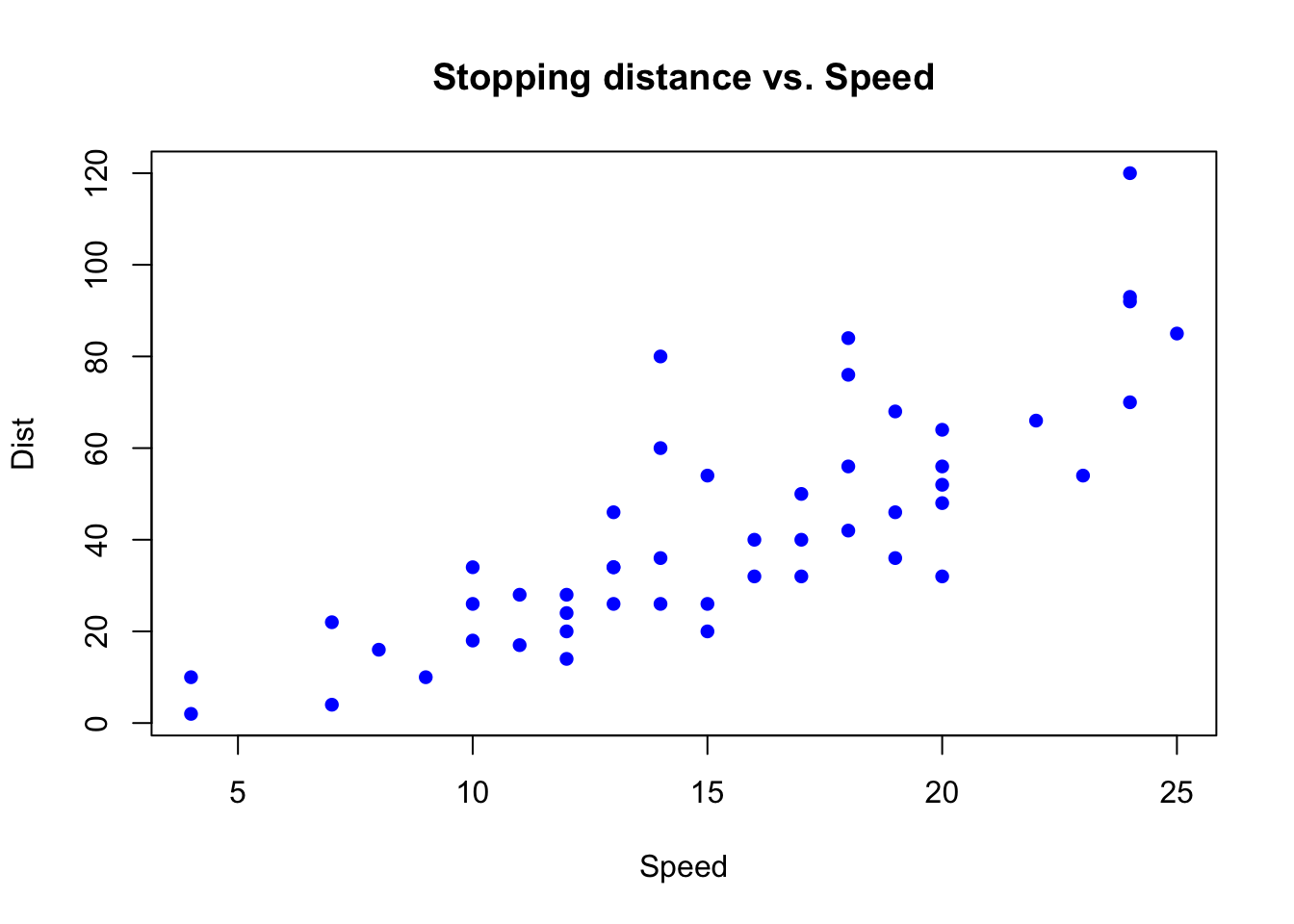 Figure 1. Scatter plot
Remember that the correlation is a measure of the linear relationship between \(X\) and \(Y\), and defined as:
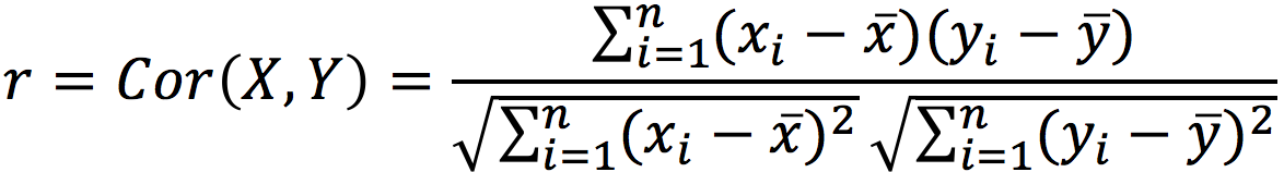
where \(\bar{x}\) denotes the mean of variable \(x\). Note that means are substracted to find the variances and the covarience. Now, lets recall the formulas used for computing the \(R^2\):
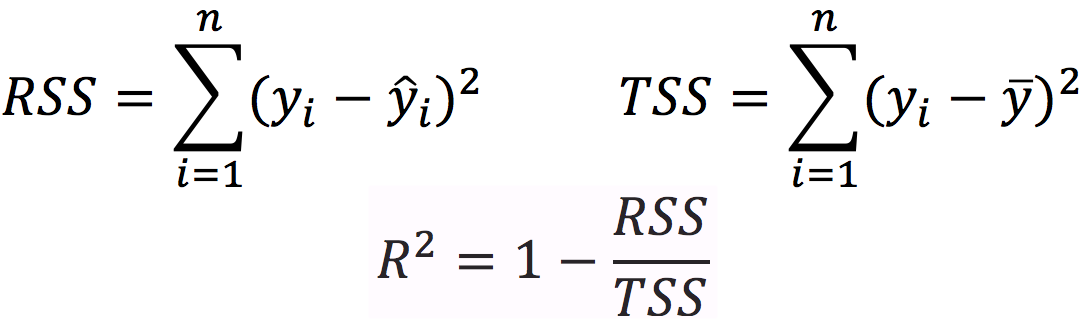
where \(RSS\) is the Residual Sum of Squares, \(TSS\) is the Total Sum of Squares, \(y\) is the obervations, \(\bar{y}\) denotes the observation mean, and \(\hat{y}\) is the predictions.
Let’s use the cor() and lm() functions to compute the \(r\) and \(R^2\), respectively:
attach(cars)
r = cor(dist,speed)
lm.fit = lm(dist~speed)
Rsquared = summary(lm.fit)$r.squared
# Print results
cat("Correlation coefficient = ", r)
## Correlation coefficient =  0.8068949
cat("Square of corr. coef. = ", r*r)
## Square of corr. coef. =  0.6510794
cat("Coefficient of determination= ", Rsquared)
## Coefficient of determination=  0.6510794
As you can see, \(r^2\) and \(R^2\) are exactly the same thing! We took the advantage of linear model object to fetch the \(R^2\), but we can verify the result using the formula:
y = dist
y_hat = fitted.values(lm.fit)
y_bar = mean(y)
RSS = sum((y-y_hat)^2)
TSS = sum((y-y_bar)^2)
Rsquared = 1 - RSS/TSS
cat("Coefficient of determination= ", Rsquared)
## Coefficient of determination=  0.6510794
Our goal was to measure the similarity between the variables \(x\) (speed) and \(y\) (distance), and we did that in two ways: First, finding the correlation between \(x\) and \(y\) and second, by modeling the linear relationship between \(x\) and \(y\). We conclude that \(r^2 = R^2\) holds for simple linear regression and when the intercept term is included. By the way, this can not be generalized to Multiple Linear Regression (please see An Introduction to Statistical Learning for more).
When \(r^2\) is NOT equal to \(R^2\)
1. If there is no constant term (intercept)
Now, let’s exclude the intercept term and see what happens. Below is a picture of fitted lines with and without the intercept term:
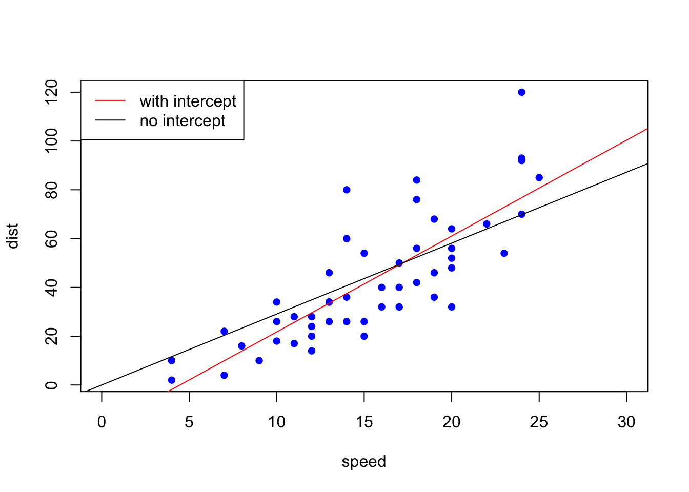
Figure 2. Fitted line with and without the intercept
Let’s take a look at the \(R^2\) one more time:
lm.fit = lm(dist ~ speed -1) # Linear fit without intercept
Rsquared = summary(lm.fit)$r.squared
cat("Coefficient of determination= ", Rsquared)
## Coefficient of determination=  0.8962893
It is different, and it is overestimated. Why? You can look here for a detailed discussion, but in simple terms, when intercept is excluded, the algorithm considers the observation mean (\(\bar{y}\) ) as 0, and thus the \(TSS\) term becomes larger leading to an increase in the \(R^2\) value.
2. If you want to explain a variable using a second variable
Now, we are going to look at the same data from a different perspective.
I am going to use the same dist and speed variables, but in a hypothetical setting. Let’s assume that I have bunch of other drivers and attributes of those drivers. I trained a model that takes driver attributes as inputs and produces the time that driver spent in traffic as the output. I tested my model on a test set (50 cars) and recorded the predicted output (\(y\_hat\)). I already know the actual output (\(y\)). Now, I want to evaluate the performance of my model. Let’s assume that \(y\) is identical to dist and \(y\_hat\) is identical to speed.
In other words, I have an actual signal and a predicted signal which happen to have the same values as dist and speed, respectively. But, we will pretend that they both have the same unit (e.g. seconds):
y <- dist
y_hat <- speed
As the performance criteria, I decided to report the similarity between the actual signal and predicted signal. Which one should I pick, \(r\) or \(R^2\)?
If we plot them on the same graph, we will see that they are quiet different from each other. Notice that x-axis is just the sample number:
x=1:50
plot(x, y, type="b", pch=19, col="red", xlab="sample no", ylab="time (min)")
lines(x, y_hat, type="b", pch=19, col="blue")
legend(1, 110, legend=c("actual", "predicted"), col=c("red", "blue"), lty=1:1)
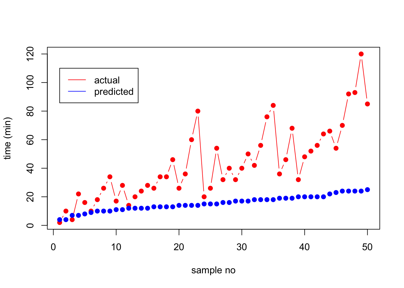
Figure 3. Original and predicted vectors
And the \(R^2\) is:
y_bar = mean(y)
RSS = sum((y-y_hat)^2)
TSS = sum((y-y_bar)^2)
Rsquared = 1 - RSS/TSS
cat("Coefficient of determination= ", Rsquared)
## Coefficient of determination=  -0.8798069
As these two signals become more separated, the \(R^2\) value will decrease while the \(r\) value will stay the same. Let’s look at this in a picture form:
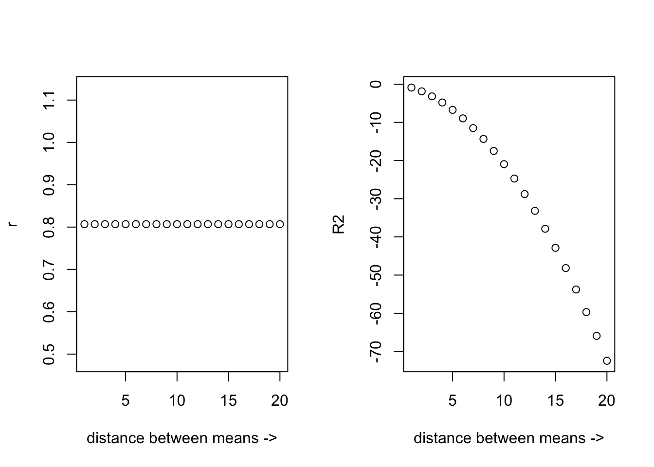
Figure 4. The \(r\) and \(R^2\) as a function of mean difference
\(R^2\) gives us a measure on how much of the variation in the actual variable \(y\) can be explained by the predicted variable \(y\_hat\). By switching their roles, we change the \(RSS/TSS\) term, thus we obtain a different \(R^2\) value.
y <- speed
y_hat <- dist
y_bar = mean(y)
RSS = sum((y-y_hat)^2)
TSS = sum((y-y_bar)^2)
Rsquared = 1 - RSS/TSS
cat("Coefficient of determination= ", Rsquared)
## Coefficient of determination=  -43.64745
To put the above phenomena into a context, let’s say that we built a model using the training data we have. But, in actuality, the features are not capable of establishing a linear relationship to the output, and it turned out that our model did a terrible job in making predictions from unseen data. Let’s say the model produced a prediction that is hugely diverted from the true values. In theory, we can still have a moderate correlation between predicted and actual signals, however, \(R^2\) will generate a very small or negative value depending on the differences in their means.
Conclusion
-
If we use Linear Regression to assess the similarity between \(x\) and \(y\), the algorithm will use y and fitted values (\(\beta_0 + X*\beta_1\)) to compute the \(R^2\). In that case, the the squared correlation and \(R^2\) will be the same.
-
If we have two separate variables (e.g. actual signal vs. the model output) and we want to compare them, we should avoid using Linear Regression function
lm()just because it automatically reports the \(R^2\). We are not interested in fitting two variables, but we want to know if our prediction is close to the actual data or not. In that case, we should directly implement the \(R^2\) formula.