Data Science Q&A

1. What are the “components of learning” in Machine Learning?
2. What is bias-variance tradeoff?
3. How is KNN different than k-means clustering?
4. What are ROC and AUC?
5. What is a cost function?
6. What is gradient descent?
7. Why feature scaling is important before applying a learning algorithm?
8. What is Linear Regression?
9. What is Polynomial Regression?
10. What is Logistic Regression?
11. Can Logistic Regression be used for multiclass classification?
12. What is overfitting? How can you avoid it?
13. What is Regularization?
14. Why is Bayes’ Rule is useful in spam filtering?
15. Does getting more training data always improve the performance of the model?
16. How do you approach a machine learning problem?
17. What type of error metrics do you use to evaluate imbalanced classifications?
18. What is SVM and how does it work?
19. How does k-means clustering algorithm work?
20. What is the “ceiling analysis” and why is it important?
21. What are the different types of testing?

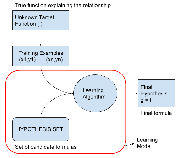
Q1. What are the “components of learning” in Machine Learning?

Consider the following diagram: (source: caltech)

• \(f\): The target function is the true function that connects the input to the output. Learning Algorithm’s goal is estimate this function to the best of its ability.

• Training examples is the historical data that is available to us. We will use this to come up with a function.

• Hypothesis set is the set of functions we choose to use. We are going to find a hypothesis \(g\) which approximates to the real hypothesis \(f\).

• Learning algorithm is the process of figuring out the hypothesis \(g\). This is when the parameters of the candidate function is decided and fine tuned.

• Hypothesis set: Linear Regression -> Learning algorithm: Ordinary least squares
  Hypothesis set: Neural Networks -> Learning algorithm: Back propagation

Q2. What is bias-variance tradeoff?

What do we mean by the variance and bias of a statistical learning method? Variance refers to the amount by which \(\hat{f}\) (function that defines the model) would change if we estimated it using a different training data set. Since the training data are used to fit the statistical learning method, different training data sets will result in a different \(\hat{f}\). But ideally the estimate for \({f}\) should not vary too much between training sets. However, if a method has high variance then small changes in the training data can result in large changes in \(\hat{f}\). In general, more flexible statistical methods have higher variance.

On the other hand, bias refers to the error that is introduced by approximating a real-life problem, which may be extremely complicated, by a much simpler model. For example, linear regression assumes that there is a linear relationship between Y and X1, X2,…,Xp. It is unlikely that any real-life problem truly has such a simple linear relationship, and so performing linear regression will undoubtedly result in some bias in the estimate of \({f}\).

Q3. How is KNN different than k-means clustering?

KNN is a supervised classification algorithm which requires labeled output to work. K refers the number of neighbors of a point. We look at these point to decide which class the point belongs to. If K is small, it means that our different classes have sharp boundaries and resulting model is probably overfitted. If K is big, the boundaries are smoother and the model is probably more generalizable.

K-means, on the other hand, refers to an unsupervised learning algorithm. It doesn’t require labelled outputs. What we need is the number of clusters that we want the points fall into, and a distance measure. The algorithm gradually finds cluster centers and a number of points around them. And concludes that these points belong to the same cluster.

Q4. What are ROC and AUC?

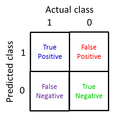
In a classification problem, the confusion matrix represents the performance of the classification algorithm. Ideally, we would like to have less misclassifications. However, depending on the decision threshold we use, the correct classifications may differ from one class to other. The ROC (receiver operating characteristic) curve is a visual representation of all the confusion matrices we have for various thresholds (for binary classifications). It helps us to decide the best threshold for our problem. The AUC (area under the curve) summarizes the ROC curve with a single value. Usually, the higher the AUC the better.

Q5. What is a cost function?

Examine the following picture (credit to Andrew Ng at Coursera):

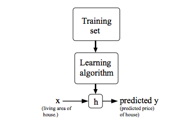
For a given training set, the learning algorithm estimates a function \(h\) (hypothesis), which maps the input to the output to the best its ability. This mapping may not be perfect, but it is the closest approximation to the actual function.

Learning algorithm tries to find the best \({Q}\) parameters. In other words, it needs to choose parameters so that \(h_{Q}(x)\) will be close the \({y}\) for our training examples. This is essentially an optimization problem and can be formulated as:

The above \(J\) is called an objective function or cost function, and can be read as the following: We have to choose \(Q_0\) and \(Q_1\) parameters that minimizes the solution to above equation. \(x^{(i)}\) denotes the \(ith\) training input.

This is sometimes called “Squared difference cost function” and it is the most commonly used cost function in regression problems.

Q6. What is gradient descent?

Gradient Descent is an algorithm that is used to minimize a function. For example, \(J(Q_0, Q_1)\) can be minimized over \(Q_0\) and \(Q_1\). Having 2 parameters, we will end up with a 3D surface function where x-axis is \(Q_0\), y-axis is \(Q_1\), and the z-axis is the output of the function.

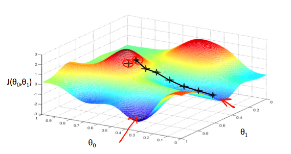
Imagine it as a landscape with hills and valleys. What Gradient Descent does is, it starts from an arbitrary point in the landscape, and finds the direction of the steepest descent at that point. After finding it, it descends with a certain distance. Then, looks for the steepest descent at the new point and jumps at that direction. It repeats this process until it reaches to a local minima. The result may not be the optimal solution, since Gradient Descent doesn’t guarantee to find the global minimum.

\(Q_j := Q_j - \alpha\frac{\partial}{\partial Q_j}J(Q_0, Q_1)\) (for \(j=0\) and \(j=1\))

\(\alpha\): learning rate (how fast the algorithm updates)

Gradient Descent is an iterative process and it is not deterministic. After each iteration, the cost function has to decrease. After a certain number of iterations, the decrease slows down and this is when you decide if the algorithm is converged or not. Usually, if you choose a very large \(\alpha\), the algorithm can overshoot and never converge. If the \(\alpha\), then you have a very slow convergence. A good practice is trying different values of \(\alpha\) and plotting the cost function to see if it is converged.

Rather than using Gradient Descent, the parameters can be computed numerically using the normal equation method:

Since normal equation method involves inverting matrices, if the number of features too large Gradient Descent would be the better choice.

Q7. Why feature scaling is important before applying a learning algorithm?

If there is a large difference between the ranges of the features, the Gradient Descent algorithm can take a long time to converge. There would be unnecessary oscillations due to highly skewed values. So, feature scaling is needed for the Gradient Descent to efficiently work.

Q8. What is Linear Regression?

Linear regression is an analytical technique used to model the relationship between several input variables and a continuous output variable. The key point is that we assume that the relationship is linear. This is a safe assumption because in the worst case, a linear relationship can be achieved by transforming the variables. Linear regression generates a probabilistic model, where some randomness always exists. Consider the following equation:

The model represents the relationship between the income (output) and age and education (input) of employees that work in a company. The error term captures the variations that do not fit the linearity assumption. The fitted model should minimize the overall error between the model output and the actual observations. But what \(\beta\) parameters should we choose to achieve this? Ordinary Least Squares (OLS) is the most commonly used technique to find those parameters. For a dataset with \(n\) observations:

Q9. What is Polynomial Regression?

If fitting a straight line to data is not applicable, maybe a more flexible line would work better. Polynomial regression provides this flexibility. It is similar to linear regression except that the cost model includes higher order versions of the features.

Q10. What is Logistic Regression?

Logistic Regression is used to solve classification problems and it is widely used by ML community. It is an extension of the Linear Regression method where the objective is fitting a linear line to a set of data points. However, using Linear Regression for a classification problem has many disadvantages. Thus, Logistic Regression has been developed as a remedy. The most obvious difference is that Logistic Regression forces the output to be somewhere between 0 and 1.

Logistic regression: \(0 \leq h_Q(x) \leq 1\)

In order to constrain the output, we use a special function, called sigmoid or logistic function. This is where the name comes from.

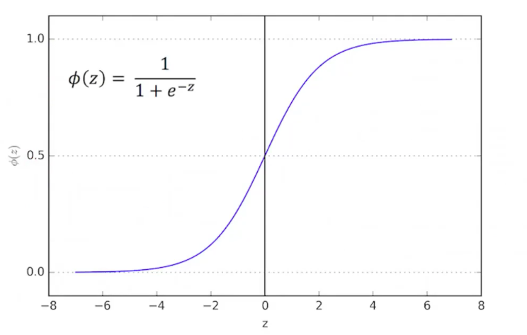
Logistic regression gives us the probability of \(h_Q(x)\) being either 1 or 0. Assume that we pick the threshold as 0.5. If the hypothesis is less than 0, logistic function leads to 0. If the hypothesis is larger than 0, the logistic function generates a 1.

Q11. Can Logistic Regression be used for multiclass classification?

Yes. Using the idea of one-vs-all, we can use standard Logistic regression to perform multiclass classification. One-vs-all treats a class as the positive class while treating all the others as negative. And repeats this for each of \(k\) classes and ends up with \(k\) number of classifiers.

Q12. What is overfitting? How can you avoid it?

High bias: Our opinion about the model is biased, e.g. we think that there is a linear relationship underlying the model, thus we use a simple linear regression model. However, the real relationship is more complex, and we underfit the curve.

High variance: We pick a complex model to fit to the training set. We do a good job but if the underlying mechanism has a lot of variance, it means that our model would not be able to capture all and it would not do a good job on a different set of data. In other words, it will overfit to the training set, but it won’t generalize.

There are two main ways to avoid overfitting:

1. Reduce number of features:
   • Either manually select the most important features and discard the noise which lead overfitting
   • Or use a feature selection algorithm to automatically eliminate least significant features
2. Regularization
   • Keep all the features, but reduce the influence of some parameters

Q13. What is Regularization?

Most of the time, in order to decrease the variance and increase model’s generalizability we want to reduce the number of features. One method is keeping all the featues in the model while decreasing their weights by shrinking them towards zero. Sometimes they are shrunken down to exactly zero. This is called regularization. Regularization plays an important role in high-dimensional datasets. We basically penalize the loss function by adding an extra term. This extra term depends on the feature weights, the higher the weights the more we penalize the loss function. Remember the cost function for linear regression. Here is the version with added regularization term:

\(\lambda\) is called the regularization parameter

Ridge regression: Regularized linear regression model. It doesn’t enforce coefficients to be zero, it only shrinks them towards zero.

Lasso regression: Similar to Ridge but it enforces the coefficient towards zero and effectively gets rid of them. It is basically a feature selection method.

Elastic net regression: In order to get the best of both worlds, this method linearly combines L1 and L2 penalties of the lasso and ridge methods.

Q14. Why is Bayes’ Rule is useful in spam filtering?

It is estimated that 60% of the emails in the world are spam. Email clients run a program in the background to classify a new email as spam or safe. One popular method is to use the words that appear in the email content to detect if it is spam or not. I mathematical terms, we are interested in the probability of en email being spam given the words inside:

Bayes’ rule can be used to compute this probability:

\(P(spam)\): The probability of an email being spam, regardless of the words it contains. According to our experience, this number is 60%. \(P(words|spam)\): How often these words are seen when the email is classified as spam? \(P(words)\): How often this word combination is used regardless of spam.

The classification algorithm used here is called Naive Bayes Classification. The “naive” part comes from the classifier’s assumption that features are independent; knowing one feature doesn’t tell us anything about the other features. This is a naive assumption because in reality, most of the time the features are dependent.

Q15. Does getting more training data always improve the performance of the model?

If you have few data points, the model will be trained easily since there is less points to be fitted. As the training data increase, fitting those data points will get progressively harder. On the other hand, the more training data you have the better chance there is for your model to generalize. There are two extremes that you have to consider:

1) High bias (simple model, underfitting)

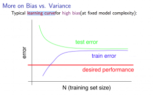
If a learning algorithm is suffering from high bias, getting more training data will not (by itself) help much.

2) High variance (complex model, overfitting)

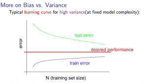
If a learning algorithm is suffering from high variance, getting more training data is likely to help.

Q16. How do you approach a machine learning problem?

Rather than relying on your gut feeling and randomly trying different methods to optimize your learning algorithm, you can take the following steps to make informed decisions:

1. Start with a simple model. Use training, validation, and test sets to evaluate your model. Slowly build up your model to a more complex version.

2. Plot learning curves and try to see if you have a high bias problem (your model is too simple) or high variance problem (your model can’t generalize to unseen data). Then, take an appropriate action to improve your model.

3. Perform error analysis. Manually examine the samples your model got wrong. See if there is any pattern to it. Think what type of features is causing the confusion and which ones are helping. Try to add new features that might have caught those errors.

Q17. What type of error metrics do you use to evaluate imbalanced classifications?

We can use precision and recall. We want them to be close to 1 for high performance classifiers.

For example:

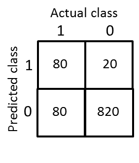
Interpretation: If we were to use the good-old misclassification metric, accuracy, the above classifier actually performed very good, i.e. 90%. However, in reality, half of the positive class is misclassified. So, this classifier does a terrible job and recall captures that. But, when it assigns a positive class its decision is correct 80% of the time, and precision captures that information. Using these two metrics, we can report the classification performance with a single numerical number, that is called F1 score:

This number should be close to 1 for us to conclude that this is a good classifier. As you can see, 0.6 is not good enough.

Q18. What is SVM and how does it work?

SVM stands for Support Vector Machines, and “it is arguably the most successful classification method in machine learning” (Prof. Abu-Mostafa).

Consider the following dataset:

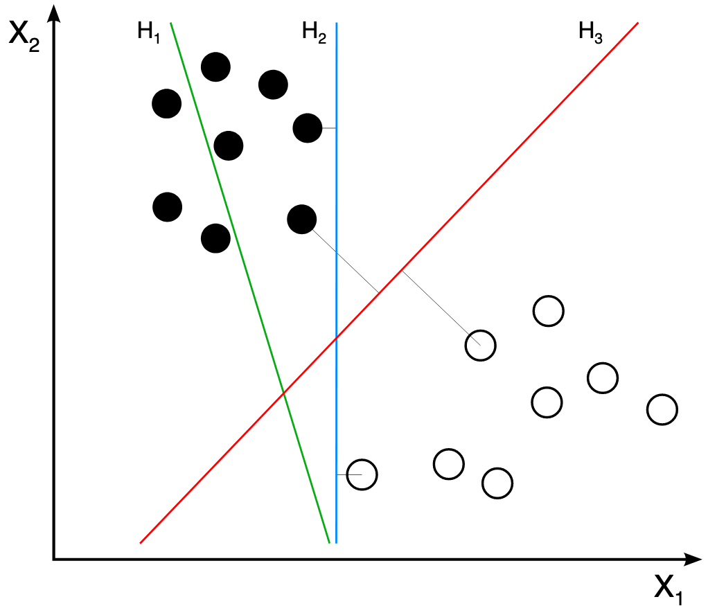
• Which line best separates the two classes? H1 doesn’t separate the classes. H2 does, but only with a small margin. H3 is the best line, separates with the highest margin. But, how do we find H3, how do we decide the best line?

• The distance from the separating line corresponds to the confidence of our classification. The farther a point from the line, the more confident we are that it belong to its class. An SVM performs classification by finding the hyperplane that maximizes the margin between two classes. The vectors that define the hyperplane are the support vectors.

• SVM performs a constrained optimization problem. The optimization is to maximize the distance between the nearest points in classes and the hyperplane (margin), and the constraints are the nearest data points should not fall inside the margin.

• When using an SVM model, there are few parameters to consider:
  • \(C\) constant: This parameter adjusts the complexity of the model. If you pick a large C, the decision boundary would become more curvy and lead overfitting.
  • Kernel trick: If the classes are not linearly separable, i.e. if there is a need for a nonlinear decision boundary. We can use the kernel trick to transform the data into a linearly separable space.
  • \(\sigma^2\): This parameter is the variance in the Gaussian kernel. The larger it is, the wider the gaussian curve (smooth kernel, simple model, leads high bias).
• Which one to use? Logistic regression or SVM? \(m\): number of observations, \(n\): number of features.
  • \(n\) is large (10,000), \(m\) is small (10-1,000): Use Logistic Regression or SVM with linear kernel. (you don’t have enough data to figure out the complexity in the data)
  • \(n\) is small (1 - 1,000), \(m\) is intermediate (1,000 - 10,000): Use SVM with Gaussian kernel. (seems a fairly complex dataset, better use Gaussian kernel)
  • \(n\) is small (1 - 1,000), \(m\) is large (50,000+): Try to add more features and use Logistic Regression or SVM without a kernel.

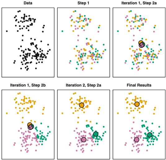
Q19. How does k-means clustering algorithm work?

(From Hastie & Tibshirani). K-means clustering is a simple and elegant approach for partitioning a data set into K distinct, non-overlapping clusters, such that the total within-cluster variation, summed over all K clusters is as small as possible. The algorithm flows as follows:

1. Randomly assign a number, from \(1\) to \(K\), to each observations. These serve as initial cluster assignments for the observations.

2. Iterate until the cluster assignments stops changing:
   a) For each of the \(K\) clusters, compute the cluster centroid. The \(kth\) cluster centroid is the vector of the \(p\) feature means for the observations in the \(kth\) cluster.
   b) Assign each observation to the cluster whose centroid is closest (where closest is defined using Euclidean distance)

Note: Because the K-means finds a local rather than a global optimum, the results depend on the initial random class assignments. For that, you should run the algorithm multiple times and select the best solution (in which the objective function is minimized). See the picture to visualize the steps.

Q20. What is the “ceiling analysis” and why is it important?

Ceiling analysis is the process of identifying the weakest (and most promising) link in your machine learning pipeline which is worth to improve. Your machine learning pipeline might compose of multiple components each performing a different task. If your pipeline is performing poorly in overall, which part of the pipeline you should work on so that its performance improves?

Let’s assume that we have the following ML pipeline for a car detection application:

• image -> 80% (overall accuracy)
• background removal -> 90% (receives 100% correct labels)
• image segmentation -> 92% (receives 100% correct labels)
• vehicle recognition -> 100% (receives 100% correct labels)

Let’s assume that we want to use ceiling analysis to identify the bottlenecks in our system. What we do is we manually label the test set for a particular component (background removal), so that that components receives 100% correct labels. Then, we check the system’s performance. If there is a large increase, for instance from 80% to 90%, then it means that correctly labelling the test set at that component is very important and we should invest our time to improve that component.

Q21. What are the different types of testing?

There are 3 test classes:

1. Unit testing
   • validate each piece of program
   • each function is tested separately
2. Regression testing
   • running the unit test again after fixing bugs
   • this is to ensure that you didn’t introduce new bugs
3. Integration testing
   • test the whole system
   • make sure that interacting pieces work nicely